
On this page
A fuel-level resistor card cannot be selected from tank capacity or end resistance alone. The card sees the motion delivered by the float and linkage, while the gauge or controller sees a loaded electrical network. Tank shape, reserve definition, arm geometry, mechanical stops, wiper path and receiver input can each introduce a different nonlinearity. This guide turns those interfaces into a selection record. The separate calibration-method owner explains how volume targets become resistance points; this page decides what track architecture can deliver those points in the installed mechanism.
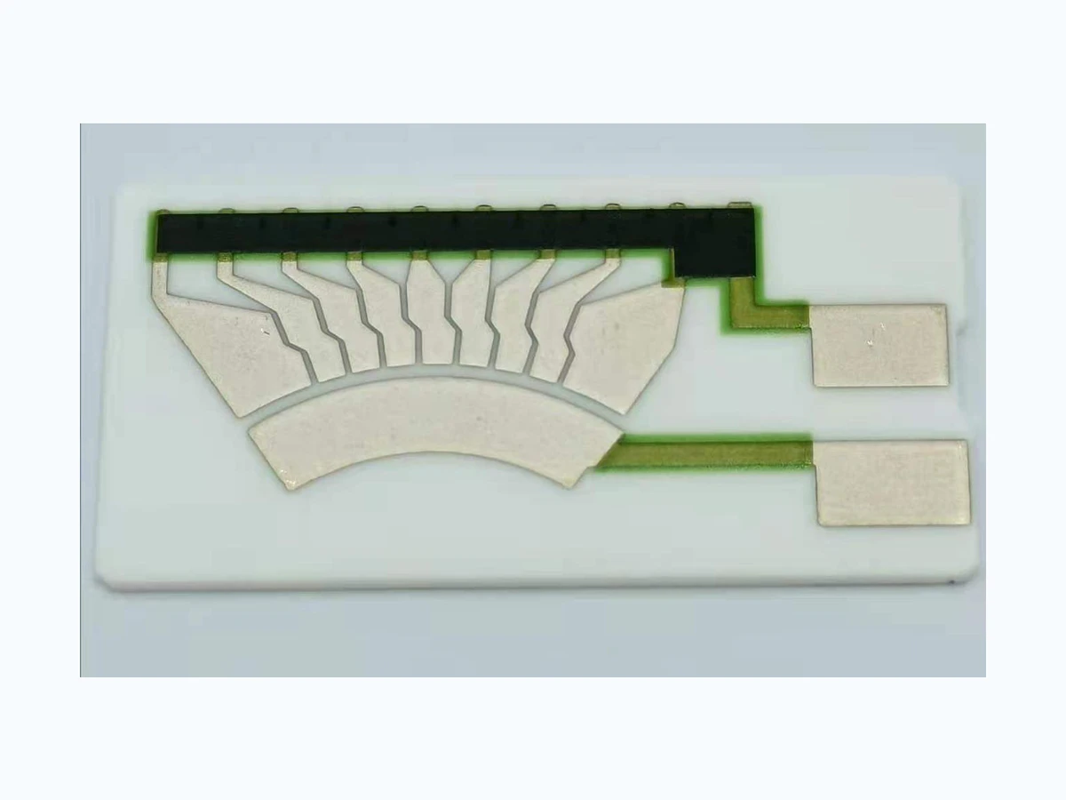
For a drawing-specific part, review the Fuel level sensor resistor card construction, product evidence and quotation inputs alongside this method. Prepare the curve and error worksheet with your operating conditions.
Key design decisions
- Freeze the usable volume-height-travel point table and the mechanical datum before choosing a printed curve.
- Calculate the loaded receiver output, including pull-up or pull-down resistance, lead resistance and diagnostics, instead of judging the card by unloaded resistance only.
- Select the track segmentation, active span and validation plan from bidirectional installed-system sweeps, not from a generic linear card.
Start with one controlled conversion chain
The selection input is a revision-controlled table linking usable volume, liquid height, float position, shaft angle or linear travel, and required receiver indication. Each column needs units and a datum. Empty may represent a reserve condition rather than a dry tank; full may be limited by expansion volume or fill geometry. Retain those definitions so a later change in tank policy is not misdiagnosed as a resistor-card error. Points that the linkage cannot reach are removed or the mechanism is revised before track artwork begins.
This page does not recreate the tank model. It checks whether the resulting travel-to-electrical requirements are monotonic, physically reachable and sufficiently separated for the intended receiver. Identify fill and drain directions because float friction, linkage clearance and liquid forces can produce different positions at the same nominal volume. If the system expects one value in both directions, the permitted hysteresis belongs in the system acceptance record rather than being silently absorbed into the printed curve.
Fit the active track to real motion and stops
Locate pivot, card and wiper from shared mechanical datums. Define the first and last valid contact positions, active travel, inactive landing zones, overtravel, assembly tolerance and contact footprint. A stop that permits the wiper to leave the resistive or collector region can create an open circuit even when the nominal calibration curve is correct. Conversely, extending active material under a stop does not guarantee useful output if contact force or alignment is uncontrolled there.
Check the contact trajectory across the entire tolerance stack. Arc radius, shaft eccentricity, carrier position, arm compliance and card mounting can shift the footprint radially and angularly. Reserve edge margin based on the real footprint rather than its centerline. A nonlinear electrical response can be printed along a mechanically simple arc, but it cannot repair intermittent contact, backlash or unreachable travel. Those mechanical effects require assembly control and bidirectional measurement.
Model the receiver that loads the sender
State whether the card is used as a two-terminal variable resistor, a three-terminal divider or a segmented contact network. Provide supply, pull-up or pull-down value, source resistance, receiver impedance, ADC range, diagnostic currents, connector and lead resistance, and the terminal reference. A resistance-versus-angle table alone is ambiguous when the receiver converts it through another network. The same card can produce different voltages when loading or wiring changes.
For a divider with upper segment R1 and lower segment R2, an ideal high-impedance receiver gives Vo equal to Vs multiplied by R2 divided by R1 plus R2. With a finite receiver resistance RL to ground, replace R2 by its parallel combination with RL. Add stable lead or contact terms at their actual circuit locations. Do not hide variable contact resistance inside a curve polynomial; preserve it as a separate error and diagnostic contributor.
Vo = Vs × (R2 || RL) / [R1 + (R2 || RL)]; R2 || RL = R2RL/(R2 + RL)
- Vs is the stated excitation voltage.
- R1 and R2 are the track resistances on either side of the wiper at one mechanical position.
- RL is the receiver resistance connected across the lower segment in this example.
- Vo is the loaded receiver voltage before ADC and software conversion.
The example is a static resistive divider; wiring topology, diagnostics, filtering and contact behavior must match the project schematic.
Quantify a receiver-loading error before choosing the curve
Take a hypothetical 5 V divider with R1 equal to 250 ohms and R2 equal to 750 ohms at one travel point. With an ideal receiver, Vo is 5 multiplied by 750 divided by 1,000, or 3.75 V. If the receiver presents 10 kilohms to ground, R2 in parallel with that load is approximately 697.7 ohms. The loaded output becomes about 3.68 V. The roughly 69 mV difference is produced by the interface, not by a printing error.
Whether 69 mV matters depends on the indicated-volume tolerance, ADC scale, noise and diagnostics. It must be converted through the controlled receiver function. Changing track resistance can reduce or increase loading effects, but it also changes current, contact conditions and diagnostic thresholds. Selection therefore compares candidate curves under the complete schematic. A high-impedance bench meter is useful for card characterization but cannot stand in for the installed receiver.
| Item | Value | Selection consequence |
|---|---|---|
| Excitation | 5.00 V | Use the actual tolerance and diagnostic states |
| Track segments | R1 = 250 Ω; R2 = 750 Ω | Unloaded position fraction is 0.75 |
| Ideal receiver | Vo = 3.750 V | Reference only |
| Receiver load | RL = 10 kΩ | R2 || RL ≈ 697.7 Ω |
| Loaded receiver | Vo ≈ 3.681 V | About 69 mV below the ideal result |
| Decision | Convert through gauge/ADC function | Do not trim the card against an unloaded target |
Choose continuous, shaped or segmented output deliberately
A continuous resistive track can provide a smooth transfer, while conductor fingers over a resistive region can create controlled steps or sampling points. Track width, path length, segment pitch, terminal placement and inactive zones must match the required point table and contact footprint. Choose point density where the combined tank-mechanism-receiver map changes rapidly. Equal angular spacing is not automatically equal volume resolution.
Decide where nonlinearity is owned. It may be implemented in tank geometry mapping, printed-track geometry, discrete segments, receiver electronics or software. Two simultaneous corrections can overcompensate the same effect. The release record should state which conversion the card owns and which remains in the controller. Redundant channels, if required by the system, need independent terminal, correlation and fault-detection definitions; this guide does not assign a safety architecture to the card.
Separate curve error from mechanism and contact faults
A smooth, repeatable offset across the sweep suggests a datum, excitation or calibration issue. A difference between fill and drain traces suggests linkage friction, float behavior or backlash. A local repeatable deviation at the same angle can indicate track geometry, segmentation or a mechanical feature near that position. Short spikes, dropouts or direction-dependent noise point toward contact, contamination, vibration, connector or acquisition timing rather than a simple resistance-curve correction.
An endpoint reached on the bench but not in the tank indicates an installed stop, buoyancy or interference boundary. A curve that matches resistance measurements but not displayed volume requires review of tank mapping and receiver conversion. Preserve raw angle, resistance and voltage alongside displayed output so the error can be located. Adjusting printed artwork to compensate an unmeasured linkage fault may improve one assembly while making the controlled geometry wrong.
Verify card, mechanism and tank in increasing context
First measure the card with a controlled wiper position and the project schematic or equivalent loading. Then sweep the complete dry mechanism with an independent angle or travel reference in both directions. Finally compare installed-tank fill and drain points at the defined orientation and liquid state. Keep independent intermediate points that were not used to create the curve; matching only the calibration knots cannot reveal interpolation error between them.
The system owner defines acceptance for volume indication, endpoints, hysteresis, repeatability, contact interruptions, temperature, vibration, media, cycling and diagnostics. Record settling and filtering because slosh response and display delay are system behaviors. Use the named service fuel or an approved test medium under a controlled plan. A dry fixture can validate geometry and loading, but it does not establish fuel compatibility, float buoyancy or complete installed performance.
Release a selection record that survives system changes
Provide the card drawing with pivot datum, active and inactive spans, contact trajectory, terminals, track or segment geometry and required values at controlled positions. Attach the source volume-height-travel-resistance table and identify the receiver schematic revision. State reference temperature, excitation, direction, measurement timing, permitted curve error and separately allocated mechanical, contact and electrical contributions.
Changes to tank geometry, reserve definition, float, arm, pivot, stops, wiper, receiver loading, diagnostics or software conversion can reopen selection even when the card outline remains unchanged. Link those interfaces through revision control and preserve raw validation data. The selected card is therefore a system-specific transfer element, not a catalogue curve whose endpoints alone guarantee the installed gauge response.
Review a fuel-level sender card for the installed mechanism
Send the complete conversion chain and receiver circuit so track architecture and validation can be reviewed against the real tank system.
- Tank drawing, orientation, usable-volume definition and controlled volume-height data.
- Float, arm, pivot, stops, travel direction, tolerance stack and contact trajectory.
- Required volume-height-travel-resistance or output points with interpolation and allowable error.
- Receiver schematic, excitation, loading, ADC or gauge conversion, diagnostics and filtering.
- Card outline, mounting datums, terminals, wiper material, force and active/inactive regions.
- Fuel or approved medium, temperature, vibration, cycling and complete-system validation requirements.
The drawing-upload form loads as you reach this section.