
On this page
A probe can be electrically calibrated and fully settled while still reading away from the temperature of the region around it. Its sheath and internal conductors connect the sensing region to a different thermal environment outside the fixture. Increasing insertion changes that path, but it can also move the sensing element through a real temperature gradient. The useful engineering question is not simply whether deeper is better; it is which physical effect the depth comparison can establish.
System boundary
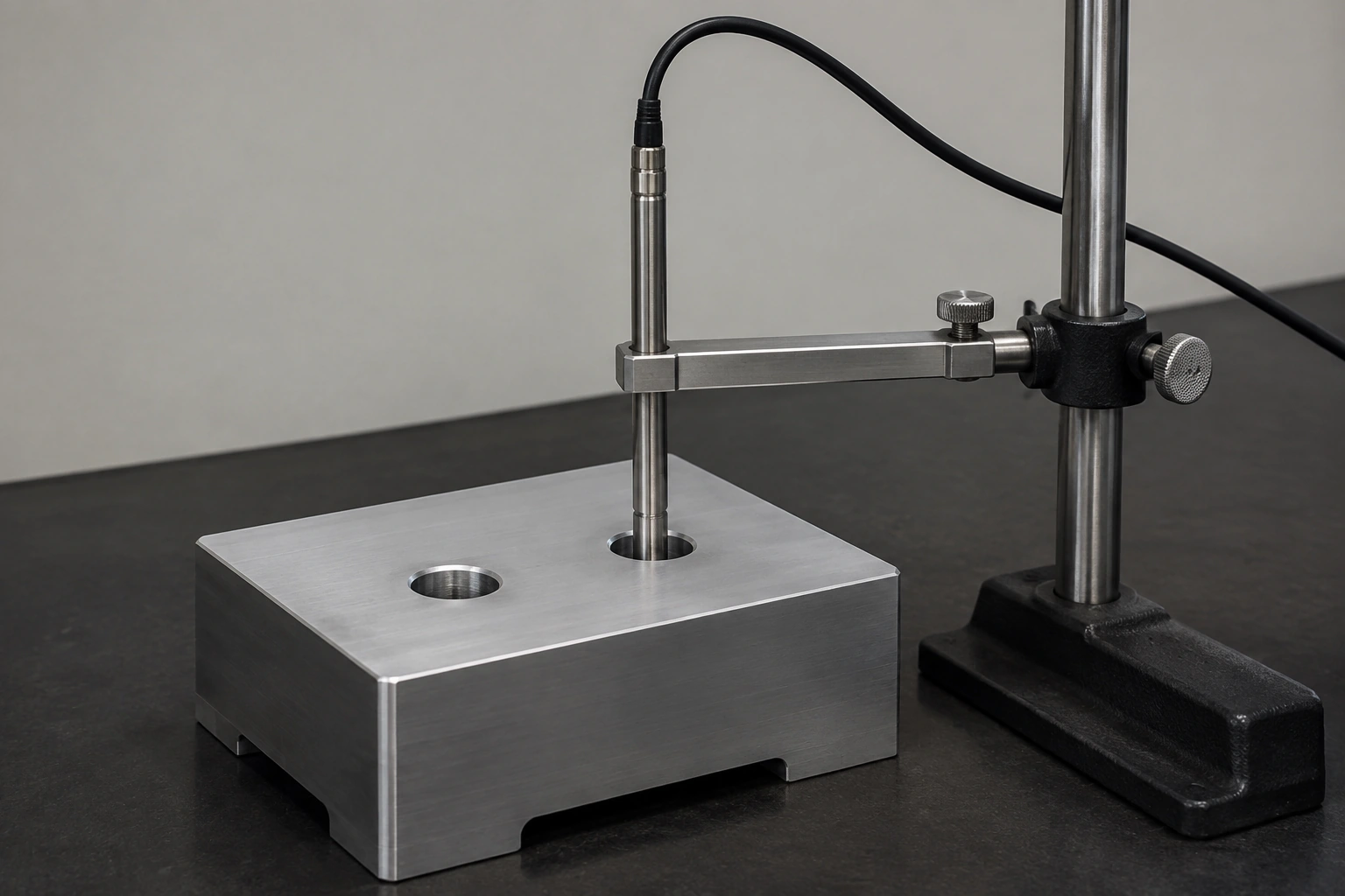
A printed heater coupled to an instrument fixture containing an inserted temperature probe. The probe, well, exposed stem and ambient boundary form the measurement installation. The instrument and metrology teams own the probe method and uncertainty; the heater construction alone does not establish temperature accuracy.
System integration decisions
- Locate the sensitive element inside the probe, not only the visible probe tip.
- Separate a depth-dependent fixture gradient from heat flow along the probe stem.
- Qualify the intended insertion and exposed-stem condition without transferring a universal minimum depth.
Dimension the sensing region rather than the metal tip
A probe drawing should identify where temperature sensitivity occurs inside the sheath. The sensitive region may have a finite length and need not start at the outer tip. Two probes seated against the same mechanical stop can therefore observe different parts of a well. Record the insertion coordinate from an accessible fixture datum and translate it to the sensitive region using the probe construction information.
If that internal location is unknown, do not silently replace it with the tip coordinate. Obtain the relevant construction information or carry the uncertainty into the comparison. A precise depth gauge cannot resolve an unknown offset between the tip and the element. This is a geometry interface, separate from the accuracy of the electrical resistance or voltage readout.
Identify the thermal path that leaves the heated region
The sheath and conductors provide routes for heat exchange with the exposed stem and its surroundings. When a heated fixture is above ambient, that path can pull the sensing region toward a lower temperature. Below ambient the direction can reverse. An immersed portion of stem that approaches the surrounding temperature reduces the driving difference near the sensing region, but the achieved result depends on the actual probe and installation.
Do not confuse this mechanism with electrical self-heating. Reducing measurement current can reduce heat generated inside a resistive sensor, but it does not remove heat conducted toward an external clamp or connector. Both effects may exist, so the investigation must identify which input it changes. Keep probe excitation fixed during a comparison intended to study the mechanical thermal path.
Use a simple balance to understand the direction of bias
A limited steady model can represent the sensing region as one temperature coupled to the target by conductance Gt and to an external thermal boundary by conductance Ge. With no internal heat generation, the indicated temperature is their conductance-weighted average. The model is useful for checking direction and sensitivity, not for calculating an insertion depth from dimensions alone.
For illustrative values Gt equal to nine times Ge, a target at 60°C and an external boundary at 20°C produce a sensing temperature of 56°C. The four-degree offset is a consequence of those assumed conductances, not an expected probe error. A changed external boundary shifts the result even though the electrical calibration is unchanged. Real distributed probes may require a more detailed model and measured validation.
Ts − Tt = [Ge / (Gt + Ge)] (Te − Tt)
- Ts is the simplified sensing-region temperature.
- Tt and Te are the target and external-boundary temperatures.
- Gt and Ge are positive effective thermal conductances to those boundaries.
Steady single-node approximation, constant effective conductances, no internal excitation heat and no separate radiative or transient term. It explains heat-path competition but does not specify a permissible installation.
Do not label every immersion curve as stem error
Changing insertion depth also changes which part of the fixture the element occupies. If the well has an axial gradient, the observed shift contains that real temperature difference. A depth sweep through an uncharacterized gradient cannot separate the two effects merely because the curve is smooth. The reference arrangement needs sufficient information about the spatial field for the intended inference.
A fixed comparison thermometer can help identify temporal movement during the sequence, but it does not automatically remove the moving probe's spatial change. Keep the gradient characterization, fixed observation and probe-depth record distinct. The measurement owner should select a comparison arrangement that can resolve the required error without assuming the heater-controlled region is perfectly isothermal.
| Mechanism | Information needed | Incorrect conclusion to avoid |
|---|---|---|
| Stem heat exchange | Exposed boundary and actual probe construction | Electrical calibration eliminates installation bias |
| Axial fixture gradient | Temperature field over the sensitive region | Every depth-dependent shift is stem conduction |
| Different element location | Internal sensitive-region position and length | Equal tip depth means equal observation volume |
| Incomplete equilibration | Time trace after the depth change | An early reading is the final immersion offset |
| Changed thermal loading | Other probes and occupied wells | The fixture field remained unchanged during the comparison |
Compare the region sensed by each probe
An element distributed over a length responds to temperatures over that region rather than to an infinitesimal point. A short element and a longer element can disagree in the same axial field even when their centers align. Do not interpret their difference as the calibration error of one probe until this spatial averaging has been considered.
Where a calculation is justified, it needs the sensitivity distribution as well as the temperature profile. A simple unweighted average is only an approximation for a suitably uniform sensitivity. Keep the model explicit and do not infer the internal distribution from the external sheath length. The practical design response may be a better-defined measurement zone or a probe construction that fits it, rather than a numerical correction based on guessed geometry.
Control the exposed stem after installation
The final cable route, support and connector position can change thermal exchange outside the well. A clamp connected to a cool chassis creates a different boundary from an unsupported probe used on the bench. Enclosure airflow or a nearby hot component can also change the external temperature. Include these features in the installed measurement drawing.
A comparison performed before the cover and cable supports are installed should not be treated as the complete instrument result. Repeat the relevant assessment in the configuration that will be used, within the equipment owner's approved conditions. If service replacement changes probe length or clamp position, the original installation record should make that change visible before a stored correction is reused.
Preserve what was held constant in the depth comparison
Keep the fixture load and the other inserted objects identified during the comparison. Adding or removing another probe changes a heat path and may alter the field being used as the observation source. Record the sequence and allow the system to reach the relevant steady condition after each authorized change; the required wait belongs to the observed installation, not a universal timer.
Returning to an earlier configuration helps reveal drift or a non-reproducible seating condition. It does not prove that the deepest reading is the true target temperature. State the remaining uncertainty and the evidence supporting the chosen operating depth. Avoid using a visually flat pair of readings as an unlimited accuracy claim when the measurement resolution or spatial field cannot resolve the required difference.
Release a defined sensing installation
The usable output is a controlled probe-and-fixture arrangement: identified probe construction, insertion datum, permitted position, exposed thermal boundary and the domain of the comparison. A minimum depth, if established, belongs to that configuration and its measurement objective. Do not extend it to a different sheath, well clearance or ambient condition without reviewing the changed heat path.
For a heated instrument assembly, provide the intended target temperature region and the sensing geometry together. The printed heater can then be reviewed against the actual thermal boundary while the metrology owner retains responsibility for the temperature indication. This division prevents controller tuning or a resistance adjustment from becoming a substitute for a demonstrated probe installation.
Provide the installed probe geometry
Connect the heater fixture drawing to the measurement region and exposed-stem conditions.
- Probe drawing with sensitive-region position, length and permitted insertion.
- Well geometry, insertion datum, other thermal loads and target measurement region.
- External stem, supports, connector location and environmental conditions.
- Depth-comparison records, spatial-field information and required measurement uncertainty.
The drawing-upload form loads as you reach this section.