
On this page
A ceramic circuit can be nearly uniform through its thickness while still having a hot region several millimeters away from a cooler terminal. High thermal conductivity does not eliminate that distinction during a short pulse. Before replacing an aluminum nitride circuit with one thermal node, compare the time available for internal diffusion with the distances separating the heat source, sensor and cooling contacts. This check determines where spatial temperature information is needed; it does not establish a product temperature limit or a guaranteed warm-up time.
Key design decisions
- Evaluate through-thickness and lateral distances separately rather than using the smallest substrate dimension for every thermal question.
- Use thermal diffusivity at the relevant material state and temperature; conductivity alone is not a transient time scale.
- Retain local heat-source and cooling geometry when deciding whether a small Biot number actually supports the proposed single-node approximation.
Locate the temperatures that must remain distinct
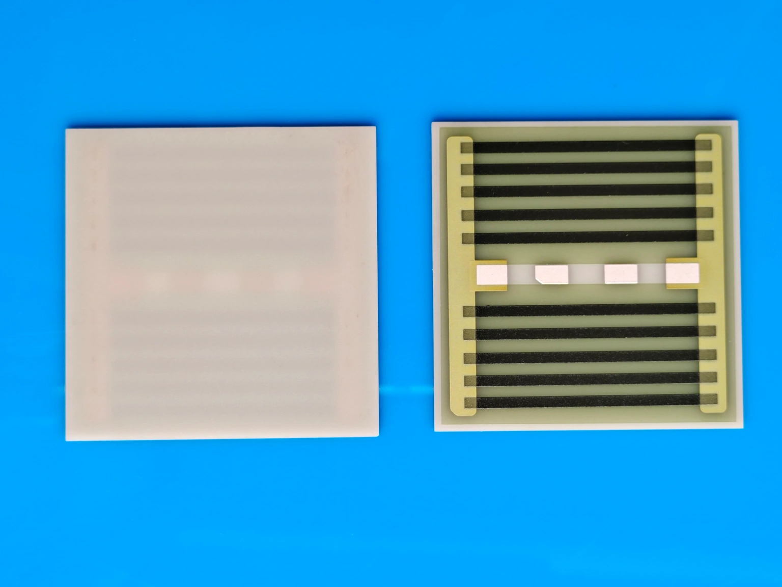
Mark the dissipating resistor or component footprint, exposed ceramic, bondline, mounting contacts and temperature measurement positions. The temperature needed for an electrical drift calculation may be the local resistor temperature, while a package requirement may concern the ceramic edge. Averaging those regions into one node can hide the temperature difference that drives the requirement.
Define the event duration as well as its power. A short pulse, a periodic pulse train and a slowly changing operating point can produce different spatial patterns in the same circuit. Record the initial thermal condition before the event. A pulse following a long idle interval is not equivalent to one occurring on an already warm board, even if voltage and current during the pulse are identical.
Form an internal diffusion time scale
Thermal diffusivity is conductivity divided by volumetric heat capacity. It describes how rapidly a temperature disturbance spreads within a material in a conduction model. For a chosen distance L, a useful scale is L squared divided by diffusivity. This scale organizes comparisons; it is not the exact time required to reach a specified temperature tolerance, which depends on shape and boundary conditions.
Use a consistent unit system. Diffusivity in square millimeters per second can be convenient when the circuit dimensions are in millimeters. Do not insert conductivity in watts per meter kelvin directly into the diffusion-time equation. If diffusivity is derived from density and heat capacity, retain the temperatures and material grade associated with those inputs. Independently mixing nominal properties from different ceramics can create an apparently precise but physically inconsistent result.
alpha = k/(rho cp); td = L^2/alpha; Fo = alpha t/L^2
- alpha: thermal diffusivity in square meters per second, or square millimeters per second when L is in millimeters.
- k: thermal conductivity in W/(m K); rho: density in kg/m^3; cp: specific heat capacity in J/(kg K).
- td: diffusion time scale in seconds; t: elapsed event time in seconds; Fo: dimensionless Fourier number for the selected L.
Homogeneous conduction with properties treated as constant over the modeled interval. The scale does not replace the spatial solution for a localized source or irregular cooling boundary.
Calculate two distances on the same hypothetical circuit
Assume a diffusivity of 60 mm^2/s solely for a numerical screening exercise. This is not a specification for an AlN grade. For a 0.5 mm through-thickness distance, the scale is 0.5 squared divided by 60, or about 0.00417 s. For a 5 mm lateral distance, it is approximately 0.417 s. A tenfold increase in distance has increased the scale by one hundred, without changing any material property.
During an assumed 10 ms pulse, the corresponding Fourier numbers are 2.4 and 0.024. The two directions are therefore at very different stages relative to their diffusion scales. It would be unreasonable to infer lateral uniformity merely because the thin direction has a larger Fourier number. Neither number alone gives the peak temperature; power density, source size and cooling conditions still determine the temperature field.
| Distance being examined | L | L squared divided by alpha | Fourier number at 10 ms | Modeling implication |
|---|---|---|---|---|
| Across the ceramic thickness | 0.5 mm | 4.17 ms | 2.4 | Through-thickness variation may be less persistent; verify the actual boundary conditions |
| From a local source to a nearby sensor | 2 mm | 66.7 ms | 0.15 | Sensor and source need not share the same transient temperature |
| From a local source toward a distant contact | 5 mm | 417 ms | 0.024 | Do not represent this lateral path as instantaneously uniform |
Use diffusion length to place the first measurements
Rearranging the same scale gives a characteristic distance equal to the square root of diffusivity times elapsed time. For the assumed diffusivity and 10 ms event, this distance is approximately 0.775 mm. Treat it as a guide to where rapid spatial changes may matter, not a sharp boundary beyond which temperature cannot change. Diffusion does not create a moving thermal front with an abrupt edge.
A temperature sensor several millimeters from a small dissipating resistor can therefore miss an early local rise. For a development comparison, choose positions close to the source and along the relevant path to the cooling contact. If the surface is observed optically, preserve enough spatial and temporal resolution to distinguish those regions. A map averaged over a large area can conceal the same gradient as a single distant sensor.
Apply the Biot check only to the boundary it represents
The Biot number compares internal conduction resistance with a boundary heat-transfer resistance. In a simple convectively cooled body, hL divided by k helps judge whether the body's internal temperature variation is small relative to its temperature difference from the fluid. The characteristic length and cooling area must belong to that body and boundary, rather than being chosen merely to make the number small.
A ceramic circuit with a tiny powered region and a bonded heat sink on part of one face is not the same problem as a uniformly cooling object in air. A small air-convection Biot number does not eliminate source-to-contact spreading gradients. Identify the actual mechanism removing the heat: convection, conduction through an attachment, edge contacts or several simultaneous paths. Use separate regions or a spatial model wherever the assumed uniform-temperature body does not match that geometry.
Keep pulse width and repetition interval separate
For repeated operation, examine both the short interval over which heat is deposited and the longer interval between pulses. The source region can experience a rapid excursion superimposed on a slowly rising background. Averaging pulse power may help estimate that background in a suitable model, but it can remove the local temperature peak that affects resistor drift or an attachment interface.
For example, changing the repetition interval while holding pulse energy fixed changes average power but leaves the individual pulse's initial spatial problem approximately similar only when the starting temperature field is also unchanged. That last condition often fails. Record several cycles until the relevant repeating behavior is established, and retain the temperature immediately before each pulse. A single cold-start record cannot establish the periodic maximum.
Test the simplification instead of only fitting one trace
A single exponential can fit a limited portion of a measured curve without proving that the whole ceramic is one thermal node. Test the proposed simplification against temperatures at more than one location and against a second pulse duration. If a fitted parameter must change substantially when the observation window moves, the model may be absorbing unresolved spatial behavior or measurement lag.
Keep power measurement synchronized with thermal capture. A delayed electrical pulse or a sensor attachment with its own time constant can imitate slow conduction. Where a multi-node model is used, require its nodes to represent identifiable regions and retain the heat-capacity and conductance assumptions. Adding enough unconstrained parameters to fit every curve does not establish that those parameters describe the actual AlN circuit.
Release the spatial model boundary with the circuit revision
The engineering output should state which temperatures are represented separately, the material-property inputs, the source and contact geometry, and the time interval over which the simplification was checked. Include the measurement positions on the same drawing coordinate system as the circuit. This makes it possible to determine whether moving a resistor, changing substrate dimensions or relocating a clamp invalidates the previous thermal representation.
If the only available result is an average temperature, do not substitute it for an unmeasured local peak. Expand the measurement or model where that peak controls the application. A successful diffusion-scale review establishes the right spatial resolution for the next thermal decision. It does not convert a substrate material property into an operating-temperature capability, a service-life prediction or a validated assembly result.
Send the transient geometry and pulse conditions
A spatial thermal review needs the distances and time scales that connect the heat source to the required temperature measurement.
- AlN grade information and the applicable conductivity, density, heat capacity or measured diffusivity with temperature conditions.
- Circuit thickness, heat-source footprint, cooling-contact map and measurement coordinates.
- Power waveform, pulse duration, repetition interval, initial temperatures and the electrical mode used to obtain the waveform.
- Local temperature limits, spatially resolved measurements, capture timing and the current thermal-model assumptions.
The drawing-upload form loads as you reach this section.