
On this page
A linear resistor track produces an electrical output along a mechanical path, but the recorded curve is limited by where it is sampled and how small an output change the receiver can distinguish. Spatial sampling pitch, digital code size, contact noise and position uncertainty are separate quantities. A useful resolution review calculates each in position units, then verifies small movements with an independent travel reference under the intended acquisition conditions.
Key design decisions
- Specify the smallest position change or local feature that must be detected before choosing sampling pitch.
- Convert converter increments and measured noise through the local output slope.
- Verify actual contact position and sample timing; motor steps and nominal converter bits do not establish achieved resolution.
Define what the system needs to distinguish
Position resolution can mean the smallest distinguishable movement, the spacing of recorded samples or the granularity of a displayed value. Accuracy describes closeness to the true position, while repeatability describes consistency under repeated conditions. State which quantity the requirement addresses and how it will be verified.
A system may record points every 0.1 millimeter while its electrical noise corresponds to 0.5 millimeter. Another may resolve small changes but carry a fixed one-millimeter offset. Neither can be summarized adequately by a single sampling-pitch number. Keep the relevant quantities separate until the complete measurement has been evaluated.
Convert motion speed and sample rate into sample spacing
For constant-speed motion, nominal spatial pitch equals speed divided by sample rate. At an assumed 20 millimeters per second and 1,000 samples per second, successive samples are 0.02 millimeter apart. This is the spacing of observations, not proof that two positions separated by that distance can be distinguished electrically.
If speed varies, calculate position from the synchronized travel reference for each sample rather than assuming constant pitch. Dropped samples, acceleration and acquisition buffering can create larger gaps. Retain actual timestamps and position data during verification. An apparently dense time series can still miss a short spatial feature if the contact moves faster through that region.
Δxsampling = v/fs
- v is contact speed in distance per second.
- fs is actual acquisition rate in samples per second.
- Δxsampling is nominal distance between samples for constant motion.
Motion is approximately uniform, samples are not dropped and timing is correctly aligned to the contact coordinate.
Convert digital increments through the local slope
For an ideal N-bit converter spanning a defined voltage range, one code interval is that range divided by two to the power N. Divide this voltage increment by the local sensor slope to obtain a nominal position increment. The converter's full input range and the sensor's used output span must not be confused.
Suppose a hypothetical sensor changes by four volts over 100 millimeters, giving 0.04 volt per millimeter. A 12-bit converter with a five-volt input range has a nominal interval of about 1.221 millivolts, corresponding to about 0.0305 millimeter at that slope. This ideal calculation excludes noise, nonlinearity, reference error and contact behavior; it is an allocation input rather than an achieved resolution.
Express measured electrical noise in position units
Measure output variation at a stationary position under the intended excitation and receiver conditions. Convert a clearly defined noise metric through the local slope. Use the same metric throughout: an RMS noise value and a peak-to-peak value are not interchangeable.
At the hypothetical 0.04-volt-per-millimeter slope, two millivolts RMS corresponds to 0.05 millimeter RMS in the simple local conversion. If the curve becomes shallower, the same voltage noise produces a larger position uncertainty. Converter noise is distinct from nominal bit count; adding output codes does not automatically improve stable position resolution.
Choose checks according to the limiting contribution
Use the calculations to identify which change would materially improve the result. Increasing sample rate helps spatial coverage, while reducing electrical noise helps distinguish output changes. Neither directly corrects mechanical uncertainty.
| Limitation | Observable symptom | Useful response |
|---|---|---|
| Spatial pitch is too coarse | Narrow features appear inconsistently between sweeps | Increase acquisition rate or reduce controlled motion speed |
| Electrical noise exceeds the required movement signal | Stationary output spans several equivalent positions | Improve the signal chain and evaluate appropriate filtering |
| Converter increment dominates | Output changes in coarse repeatable steps | Review used voltage span and converter characteristics |
| Contact position is uncertain | Electrical data repeats but absolute coordinates shift | Improve travel reference, datums or remounting control |
| Timing offset dominates during motion | Curve shifts with direction or speed | Synchronize position and output acquisition |
| Physical track has plateaus or discrete transitions | More samples reproduce the same local granularity | Review actual track structure and required local function |
Test the spatial features the sampling must capture
If the objective is to detect a narrow interruption or local curve deviation, specify its relevant width and amplitude. Choose sampling and bandwidth so that such a feature can be observed under the intended speed. A single sample within a feature may reveal an event but rarely describes its shape reliably.
Do not apply a simple two-samples-per-feature rule as a universal guarantee. Sampling theory depends on signal bandwidth and the feature model, while contact events can be abrupt and nonperiodic. Verify with an appropriate controlled signal or test structure and document the detection criterion. Preserve raw data to distinguish a missed event from filtering or display averaging.
Account for the distance traveled during filtering delay
A filter can reduce noise while delaying the response or smoothing a short event. During motion, its delay corresponds to a spatial offset equal to speed multiplied by delay. At 20 millimeters per second, an assumed 50-millisecond delay corresponds to one millimeter of travel.
Evaluate the processed output against the application's timing requirement, not only its apparent smoothness. Compare raw and filtered curves on a common coordinate and time base. If different filtering is used for calibration and operation, state the relationship. A curve calibrated from delayed data can embed a motion-dependent shift that reverses when travel direction changes.
Verify distinguishable motion with an independent reference
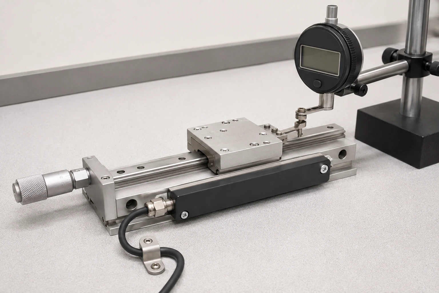
Command a sequence of small movements, measure actual position independently and record settled output distributions. Repeat in both directions and at several locations. This tests whether the desired movement produces a distinguishable change under the actual noise and mechanical conditions.
Include repeated returns to the same position to separate resolution from hysteresis and drift. For quotation, provide the smallest required movement, local error limits and acquisition method with the track drawing. The resulting review can allocate sampling, electrical and mechanical contributions realistically. A nominally continuous resistor track supports fine measurement only when the complete contact and receiver system can resolve the required output changes.
Provide the position-resolution and sampling requirements
Send the required movement scale and signal chain so spatial and electrical limits can be evaluated separately.
- Travel range, target curve and smallest position change or feature to detect.
- Local output slope, excitation and receiver voltage range.
- Actual motion speed, sample rate, timestamps and position-reference method.
- Stationary noise metric, converter characteristics and filtering delay.
- Small-step, forward/reverse and remounting results at representative positions.
The drawing-upload form loads as you reach this section.