
On this page
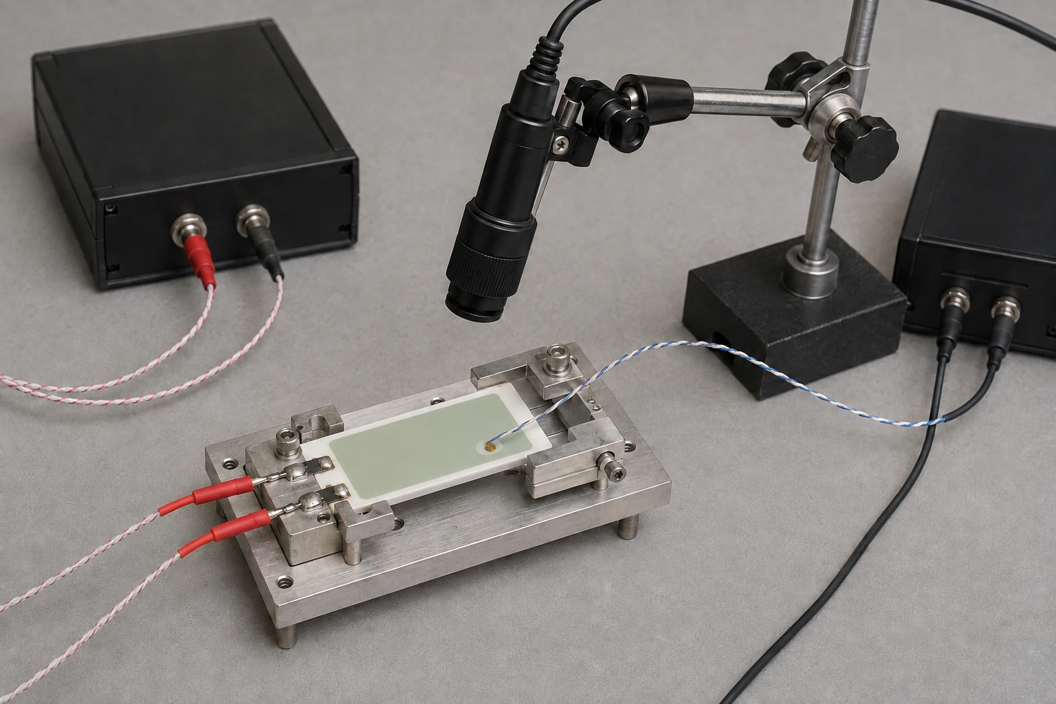
A measured ceramic temperature transient contains both the assembly's thermal response and the measurement chain's response. Fitting two time constants to that trace does not automatically reveal which belongs to the ceramic and which belongs to the sensor attachment. In a simple cascade, interchanging the two constants produces exactly the same measured curve. Resolve that ambiguity before using the fit to select a substrate, compare mounting methods or predict the unobserved heater temperature.
Key design decisions
- Separate the temperature to be estimated from the signal actually recorded.
- Treat fitted poles as unlabeled response features until independent information assigns them.
- Choose a second observation that changes identifiability, not merely another fit to the same trace.
Declare the two-stage approximation
Represent a small ceramic assembly's temperature rise above its starting condition by H, and the indicated sensor rise by S. Under a power step, let the assembly approach a final rise A with time constant tau_h. Let a first-order sensing stage follow H with time constant tau_s. Both begin at zero rise.
This cascade assumes the sensor does not significantly alter the assembly's heat flow, has unit steady temperature gain and has no separate offset toward ambient. It also assumes the assembly can be represented by one physical temperature over the evaluated interval. A heavy attached probe, a distributed ceramic gradient or significant sensor-wire heat leakage requires a different model rather than more confident fitting of this one.
Calculate what the instrument will actually record
The assembly equation is tau_h times the derivative of H plus H equals A after the step. The sensor equation is tau_s times the derivative of S plus S equals H. Solving them gives a measured response containing two exponentials rather than the single exponential of the assembly alone.
For unequal positive time constants, the normalized indicated rise is one minus [tau_h exp(-t/tau_h) minus tau_s exp(-t/tau_s)] divided by tau_h minus tau_s. The response starts at zero and approaches one. Its initial slope is zero because the assembly and sensing stage both begin at the same temperature; the physical assembly itself starts rising immediately in this model.
S(t)/A = 1 - [tau_h exp(-t/tau_h) - tau_s exp(-t/tau_s)]/(tau_h - tau_s)
- A is the final assembly temperature rise in kelvin under the stated constant power step.
- tau_h and tau_s are positive assembly and sensor response times in seconds.
- t is elapsed time from the synchronized step; S is indicated temperature rise.
Zero initial temperature rises,one-way first-order cascade,constant coefficients,unit sensor steady gain and unequal time constants.
Recognize the exact pole-label ambiguity
Interchanging tau_h and tau_s changes the signs of both numerator and denominator, leaving the complete indicated response unchanged. Perfect noiseless data for that one input-output experiment therefore cannot determine which constant belongs to the physical assembly. More samples or a tighter curve fit cannot remove this structural ambiguity.
This does not make the fitted response useless. It can describe the complete measured chain and help compare predicted indicated temperature under the same conditions. The missing information concerns the internal assignment and the unobserved physical temperature. Keep those claims separate when reporting the fit, especially if a local heater-temperature limit is the reason for the test.
Compare identical traces with different actual temperatures
Assume a final rise of 50 K. Case A has an assembly time constant of 10 seconds and a sensor constant of 2 seconds. Case B reverses them: the assembly constant is 2 seconds and the sensor constant is 10 seconds. At ten seconds both indicated rises are approximately 27.0918 K.
The actual assembly rises at that instant are very different. Case A gives approximately 31.6060 K, while Case B gives approximately 49.6631 K. The same observed 27.0918 K is compatible with either internal state under the respective model. A report that simply labels the ten-second fitted pole as ceramic response would select one explanation without evidence.
| Assumed model | Assembly constant | Sensor constant | Actual rise at10s | Indicated rise at10s |
|---|---|---|---|---|
| Case A | 10 s | 2 s | 31.6060 K | 27.0918 K |
| Case B | 2 s | 10 s | 49.6631 K | 27.0918 K |
State whether a response time belongs to the whole chain
For either case, the indicated signal reaches ninety percent of its final rise at approximately 25.2572 seconds. That is a measured-chain criterion, not either constituent time constant. A single-number report should name the fraction, starting condition, input step and observation point instead of calling every crossing time tau.
When the two constants are equal to tau, use the continuous limit S/A equal to one minus (one plus t/tau) exp(-t/tau). Directly evaluating the unequal-constant formula with identical inputs would divide by zero. At t equal to tau, this repeated-pole response has reached only approximately 26.424 percent, not the approximately 63.212 percent associated with a single first-order stage.
Choose a measurement that assigns a physical state
An independently characterized, sufficiently fast observation of the same physical region can estimate H directly and allow the original sensing stage to be evaluated against it. The comparison must represent the same region; a second sensor on a remote clamp introduces another physical gradient rather than automatically resolving the original ambiguity.
Alternatively, characterize the installed sensor response through a justified independent thermal experiment, or constrain the assembly from independently measured heat capacity and heat-removal behavior. Such information must remain applicable to the mounting and medium used in the step test. A response value from a stirred bath does not automatically identify the response of a sensor bonded through an adhesive on ceramic.
Changing the sensor or attachment deliberately can also be informative if the assembly heat path is demonstrably unchanged. If the change adds significant thermal mass or conduction, both stages may change and the comparison needs a coupled model. Document what was controlled instead of assuming the component name identifies the changed pole.
Do not confuse algebraic reconstruction with robust temperature measurement
If tau_s is independently known and the simple model is valid, the physical temperature rise satisfies H equal to S plus tau_s times the derivative of S. This identity exposes the cost of correcting lag: the derivative amplifies rapid measurement noise. Applying it to a visibly smooth plotted line can conceal the filtering and interpolation assumptions that produced that line.
For two independent samples with standard noise of 0.02 K separated by 0.1 second, a first-difference derivative has standard noise approximately square root of two times 0.02 divided by 0.1 K/s. Multiplying by an assumed two-second sensor constant gives approximately 0.566 K in the derivative contribution alone. Increasing the interval reduces this contribution but also changes the temporal approximation. This calculation is not the uncertainty of the complete reconstructed temperature.
Deliver labeled evidence, not only fitted coefficients
Retain synchronized electrical input, raw indicated temperature, independent temperature observations and the complete attachment configuration. Record which parameters came from the step fit and which came from separate measurements. Compare residual structure and repeated runs before treating the two-stage representation as sufficient.
The review conclusion should identify whether it establishes the observed chain response, a separately verified sensor constant or the physical assembly response. Preserve any unresolved assignment explicitly in the engineering model rather than using it to justify a substrate or power change. Normal process control and protective temperature observation should then be assessed against the physically supported temperature, not whichever fitted curve appears fastest.
Provide the thermal step and independent observation
Send the raw response and physical sensing arrangement so fitted dynamics can be assigned only where the measurements support that assignment.
- Ceramic assembly,heat source,sensor position,attachment and wire heat-path drawing.
- Actual power-step timing and voltage/current record with temperature timestamps.
- Initial and final thermal states,load/support conditions and the response criterion being assessed.
- Independent same-region temperature observations or separately justified sensor-response measurements.
- Raw rather than only smoothed data,filter settings,repeat runs and the proposed fitted model.
The drawing-upload form loads as you reach this section.